 Boost
C++ Libraries
Boost
C++ Libraries
...one of the most highly
regarded and expertly designed C++ library projects in the
world.
— Herb Sutter and Andrei
Alexandrescu, C++
Coding Standards
Boost
C++ Libraries
...one of the most highly
regarded and expertly designed C++ library projects in the
world.
— Herb Sutter and Andrei
Alexandrescu, C++
Coding Standards


#include <boost/math/distributions/fisher_f.hpp>
namespace boost{ namespace math{

template <class RealType = double,
          class Policy   = policies::policy<> >
class fisher_f_distribution;

typedef fisher_f_distribution<> fisher_f;

template <class RealType, class Policy>
class fisher_f_distribution
{
public:
   typedef RealType value_type;

   // Construct:
   fisher_f_distribution(const RealType& i, const RealType& j);

   // Accessors:
   RealType degrees_of_freedom1()const;
   RealType degrees_of_freedom2()const;
};

}} //namespaces
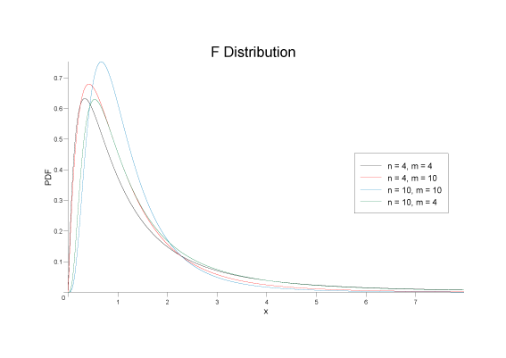
The F distribution is a continuous distribution that arises when testing whether two samples have the same variance. If χ2m and χ2n are independent variates each distributed as Chi-Squared with m and n degrees of freedom, then the test statistic:
Fn,m = (χ2n / n) / (χ2m / m)
Is distributed over the range [0, ∞] with an F distribution, and has the PDF:

The following graph illustrates how the PDF varies depending on the two degrees of freedom parameters.
fisher_f_distribution(const RealType& df1, const RealType& df2);
Constructs an F-distribution with numerator degrees of freedom df1 and denominator degrees of freedom df2.
Requires that df1 and df2 are both greater than zero, otherwise domain_error is called.
RealType degrees_of_freedom1()const;
Returns the numerator degrees of freedom parameter of the distribution.
RealType degrees_of_freedom2()const;
Returns the denominator degrees of freedom parameter of the distribution.
All the usual non-member accessor functions that are generic to all distributions are supported: Cumulative Distribution Function, Probability Density Function, Quantile, Hazard Function, Cumulative Hazard Function, mean, median, mode, variance, standard deviation, skewness, kurtosis, kurtosis_excess, range and support.
The domain of the random variable is [0, +∞].
Various worked examples are available illustrating the use of the F Distribution.
The normal distribution is implemented in terms of the incomplete beta function and it's inverses, refer to those functions for accuracy data.
In the following table v1 and v2 are the first and second degrees of freedom parameters of the distribution, x is the random variate, p is the probability, and q = 1-p.
|
Function |
Implementation Notes |
|---|---|
|
|
The usual form of the PDF is given by:
However, that form is hard to evaluate directly without incurring problems with either accuracy or numeric overflow. Direct differentiation of the CDF expressed in terms of the incomplete beta function led to the following two formulas: fv1,v2(x) = y * ibeta_derivative(v2 / 2, v1 / 2, v2 / (v2 + v1 * x)) with y = (v2 * v1) / ((v2 + v1 * x) * (v2 + v1 * x)) and fv1,v2(x) = y * ibeta_derivative(v1 / 2, v2 / 2, v1 * x / (v2 + v1 * x)) with y = (z * v1 - x * v1 * v1) / z2 and z = v2 + v1 * x The first of these is used for v1 * x > v2, otherwise the second is used. The aim is to keep the x argument to ibeta_derivative away from 1 to avoid rounding error. |
|
cdf |
Using the relations: p = ibeta(v1 / 2, v2 / 2, v1 * x / (v2 + v1 * x)) and p = ibetac(v2 / 2, v1 / 2, v2 / (v2 + v1 * x)) The first is used for v1 * x > v2, otherwise the second is used. The aim is to keep the x argument to ibeta well away from 1 to avoid rounding error. |
|
cdf complement |
Using the relations: p = ibetac(v1 / 2, v2 / 2, v1 * x / (v2 + v1 * x)) and p = ibeta(v2 / 2, v1 / 2, v2 / (v2 + v1 * x)) The first is used for v1 * x < v2, otherwise the second is used. The aim is to keep the x argument to ibeta well away from 1 to avoid rounding error. |
|
quantile |
Using the relation: x = v2 * a / (v1 * b) where: a = ibeta_inv(v1 / 2, v2 / 2, p) and b = 1 - a Quantities a and b are both computed by ibeta_inv without the subtraction implied above. |
|
quantile from the complement |
Using the relation: x = v2 * a / (v1 * b) where a = ibetac_inv(v1 / 2, v2 / 2, p) and b = 1 - a Quantities a and b are both computed by ibetac_inv without the subtraction implied above. |
|
mean |
v2 / (v2 - 2) |
|
variance |
2 * v22 * (v1 + v2 - 2) / (v1 * (v2 - 2) * (v2 - 2) * (v2 - 4)) |
|
mode |
v2 * (v1 - 2) / (v1 * (v2 + 2)) |
|
skewness |
2 * (v2 + 2 * v1 - 2) * sqrt((2 * v2 - 8) / (v1 * (v2 + v1 - 2))) / (v2 - 6) |
|
kurtosis and kurtosis excess |
Refer to, Weisstein, Eric W. "F-Distribution." From MathWorld--A Wolfram Web Resource. |