 Boost
C++ Libraries
Boost
C++ Libraries
...one of the most highly
regarded and expertly designed C++ library projects in the
world.
— Herb Sutter and Andrei
Alexandrescu, C++
Coding Standards
Boost
C++ Libraries
...one of the most highly
regarded and expertly designed C++ library projects in the
world.
— Herb Sutter and Andrei
Alexandrescu, C++
Coding Standards


#include <boost/math/distributions/negative_binomial.hpp>
namespace boost{ namespace math{

template <class RealType = double,
          class Policy   = policies::policy<> >
class negative_binomial_distribution;

typedef negative_binomial_distribution<> negative_binomial;

template <class RealType, class Policy>
class negative_binomial_distribution
{
public:
   typedef RealType value_type;
   typedef Policy   policy_type;
   // Constructor from successes and success_fraction:
   negative_binomial_distribution(RealType r, RealType p);

   // Parameter accessors:
   RealType success_fraction() const;
   RealType successes() const;

   // Bounds on success fraction:
   static RealType find_lower_bound_on_p(
      RealType trials,
      RealType successes,
      RealType probability); // alpha
   static RealType find_upper_bound_on_p(
      RealType trials,
      RealType successes,
      RealType probability); // alpha

   // Estimate min/max number of trials:
   static RealType find_minimum_number_of_trials(
      RealType k,     // Number of failures.
      RealType p,     // Success fraction.
      RealType probability); // Probability threshold alpha.
   static RealType find_maximum_number_of_trials(
      RealType k,     // Number of failures.
      RealType p,     // Success fraction.
      RealType probability); // Probability threshold alpha.
};

}} // namespaces
The class type negative_binomial_distribution
represents a negative_binomial
distribution: it is used when there are exactly two mutually
exclusive outcomes of a Bernoulli
trial: these outcomes are labelled "success" and "failure".
For k + r Bernoulli trials each with success fraction p, the negative_binomial distribution gives the probability of observing k failures and r successes with success on the last trial. The negative_binomial distribution assumes that success_fraction p is fixed for all (k + r) trials.
![[Note]](../../../../../../../../../doc/html/images/note.png) |
Note |
|---|---|
The random variable for the negative binomial distribution is the number of trials, (the number of successes is a fixed property of the distribution) whereas for the binomial, the random variable is the number of successes, for a fixed number of trials. |
It has the PDF:

The following graph illustrate how the PDF varies as the success fraction p changes:

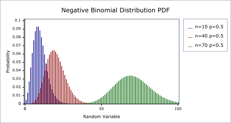
Alternatively, this graph shows how the shape of the PDF varies as the number of successes changes:
The name negative binomial distribution is reserved by some to the case where the successes parameter r is an integer. This integer version is also called the Pascal distribution.
This implementation uses real numbers for the computation throughout (because it uses the real-valued incomplete beta function family of functions). This real-valued version is also called the Polya Distribution.
The Poisson distribution is a generalization of the Pascal distribution, where the success parameter r is an integer: to obtain the Pascal distribution you must ensure that an integer value is provided for r, and take integer values (floor or ceiling) from functions that return a number of successes.
For large values of r (successes), the negative binomial distribution converges to the Poisson distribution.
The geometric distribution is a special case where the successes parameter r = 1, so only a first and only success is required. geometric(p) = negative_binomial(1, p).
The Poisson distribution is a special case for large successes
poisson(λ) = lim r → ∞ negative_binomial(r, r / (λ + r)))
![[Caution]](../../../../../../../../../doc/html/images/caution.png) |
Caution |
|---|---|
|
The Negative Binomial distribution is a discrete distribution: internally
functions like the The quantile function will by default return an integer result that has been rounded outwards. That is to say lower quantiles (where the probability is less than 0.5) are rounded downward, and upper quantiles (where the probability is greater than 0.5) are rounded upwards. This behaviour ensures that if an X% quantile is requested, then at least the requested coverage will be present in the central region, and no more than the requested coverage will be present in the tails. This behaviour can be changed so that the quantile functions are rounded differently, or even return a real-valued result using Policies. It is strongly recommended that you read the tutorial Understanding Quantiles of Discrete Distributions before using the quantile function on the Negative Binomial distribution. The reference docs describe how to change the rounding policy for these distributions. |
negative_binomial_distribution(RealType r, RealType p);
Constructor: r is the total number of successes, p is the probability of success of a single trial.
Requires: r >
0 and 0
<= p
<= 1.
RealType success_fraction() const; // successes / trials (0 <= p <= 1)
Returns the parameter p from which this distribution was constructed.
RealType successes() const; // required successes (r > 0)
Returns the parameter r from which this distribution was constructed.
static RealType find_lower_bound_on_p(
  RealType failures,
  RealType successes,
  RealType probability) // (0 <= alpha <= 1), 0.05 equivalent to 95% confidence.
Returns a lower bound on the success fraction:
The total number of failures before the r th success.
The number of successes required.
The largest acceptable probability that the true value of the success fraction is less than the value returned.
For example, if you observe k failures and r successes from n = k + r trials the best estimate for the success fraction is simply r/n, but if you want to be 95% sure that the true value is greater than some value, pmin, then:
pmin = negative_binomial_distribution<RealType>::find_lower_bound_on_p(
                    failures, successes, 0.05);
See negative binomial confidence interval example.
This function uses the Clopper-Pearson method of computing the lower bound on the success fraction, whilst many texts refer to this method as giving an "exact" result in practice it produces an interval that guarantees at least the coverage required, and may produce pessimistic estimates for some combinations of failures and successes. See:
static RealType find_upper_bound_on_p(
   RealType trials,
   RealType successes,
   RealType alpha); // (0 <= alpha <= 1), 0.05 equivalent to 95% confidence.
Returns an upper bound on the success fraction:
The total number of trials conducted.
The number of successes that occurred.
The largest acceptable probability that the true value of the success fraction is greater than the value returned.
For example, if you observe k successes from n trials the best estimate for the success fraction is simply k/n, but if you want to be 95% sure that the true value is less than some value, pmax, then:
pmax = negative_binomial_distribution<RealType>::find_upper_bound_on_p(
                    r, k, 0.05);
See negative binomial confidence interval example.
This function uses the Clopper-Pearson method of computing the lower bound on the success fraction, whilst many texts refer to this method as giving an "exact" result in practice it produces an interval that guarantees at least the coverage required, and may produce pessimistic estimates for some combinations of failures and successes. See:
static RealType find_minimum_number_of_trials(
   RealType k,     // number of failures.
   RealType p,     // success fraction.
   RealType alpha); // probability threshold (0.05 equivalent to 95%).
This functions estimates the number of trials required to achieve a certain probability that more than k failures will be observed.
The target number of failures to be observed.
The probability of success for each trial.
The maximum acceptable risk that only k failures or fewer will be observed.
For example:
negative_binomial_distribution<RealType>::find_minimum_number_of_trials(10, 0.5, 0.05);
Returns the smallest number of trials we must conduct to be 95% sure of seeing 10 failures that occur with frequency one half.
This function uses numeric inversion of the negative binomial distribution to obtain the result: another interpretation of the result, is that it finds the number of trials (success+failures) that will lead to an alpha probability of observing k failures or fewer.
static RealType find_maximum_number_of_trials(
   RealType k,     // number of failures.
   RealType p,     // success fraction.
   RealType alpha); // probability threshold (0.05 equivalent to 95%).
This functions estimates the maximum number of trials we can conduct and achieve a certain probability that k failures or fewer will be observed.
The maximum number of failures to be observed.
The probability of success for each trial.
The maximum acceptable risk that more than k failures will be observed.
For example:
negative_binomial_distribution<RealType>::find_maximum_number_of_trials(0, 1.0-1.0/1000000, 0.05);
Returns the largest number of trials we can conduct and still be 95% sure of seeing no failures that occur with frequency one in one million.
This function uses numeric inversion of the negative binomial distribution to obtain the result: another interpretation of the result, is that it finds the number of trials (success+failures) that will lead to an alpha probability of observing more than k failures.
All the usual non-member accessor functions that are generic to all distributions are supported: Cumulative Distribution Function, Probability Density Function, Quantile, Hazard Function, Cumulative Hazard Function, mean, median, mode, variance, standard deviation, skewness, kurtosis, kurtosis_excess, range and support.
However it's worth taking a moment to define what these actually mean in the context of this distribution:
Table 12. Meaning of the non-member accessors.
|
Function |
Meaning |
|---|---|
|
The probability of obtaining exactly k failures from k+r trials with success fraction p. For example:
pdf(negative_binomial(r, p), k)
|
|
|
The probability of obtaining k failures or fewer from k+r trials with success fraction p and success on the last trial. For example:
cdf(negative_binomial(r, p), k)
|
|
|
The probability of obtaining more than k failures from k+r trials with success fraction p and success on the last trial. For example:
cdf(complement(negative_binomial(r, p), k))
|
|
|
The greatest number of failures k expected to be observed from k+r trials with success fraction p, at probability P. Note that the value returned is a real-number, and not an integer. Depending on the use case you may want to take either the floor or ceiling of the real result. For example:
quantile(negative_binomial(r, p), P)
|
|
|
The smallest number of failures k expected to be observed from k+r trials with success fraction p, at probability P. Note that the value returned is a real-number, and not an integer. Depending on the use case you may want to take either the floor or ceiling of the real result. For example: quantile(complement(negative_binomial(r, p), P))
|
This distribution is implemented using the incomplete beta functions ibeta and ibetac: please refer to these functions for information on accuracy.
In the following table, p is the probability that any one trial will be successful (the success fraction), r is the number of successes, k is the number of failures, p is the probability and q = 1-p.
|
Function |
Implementation Notes |
|---|---|
|
|
pdf = exp(lgamma(r + k) - lgamma(r) - lgamma(k+1)) * pow(p, r) * pow((1-p), k) Implementation is in terms of ibeta_derivative: (p/(r + k)) * ibeta_derivative(r, static_cast<RealType>(k+1), p) The function ibeta_derivative is used here, since it has already been optimised for the lowest possible error - indeed this is really just a thin wrapper around part of the internals of the incomplete beta function. |
|
cdf |
Using the relation: cdf = Ip(r, k+1) = ibeta(r, k+1, p) = ibeta(r, static_cast<RealType>(k+1), p) |
|
cdf complement |
Using the relation: 1 - cdf = Ip(k+1, r) = ibetac(r, static_cast<RealType>(k+1), p) |
|
quantile |
ibeta_invb(r, p, P) - 1 |
|
quantile from the complement |
ibetac_invb(r, p, Q) -1) |
|
mean |
|
|
variance |
|
|
mode |
|
|
skewness |
|
|
kurtosis |
|
|
kurtosis excess |
|
|
parameter estimation member functions |
|
|
|
ibeta_inv(successes, failures + 1, alpha) |
|
|
ibetac_inv(successes, failures, alpha) plus see comments in code. |
|
|
ibeta_inva(k + 1, p, alpha) |
|
|
ibetac_inva(k + 1, p, alpha) |
Implementation notes: