 Boost
C++ Libraries
Boost
C++ Libraries
...one of the most highly
regarded and expertly designed C++ library projects in the
world.
— Herb Sutter and Andrei
Alexandrescu, C++
Coding Standards
Boost
C++ Libraries
...one of the most highly
regarded and expertly designed C++ library projects in the
world.
— Herb Sutter and Andrei
Alexandrescu, C++
Coding Standards


Let's say you have a sample mean, you may wish to know what confidence intervals you can place on that mean. Colloquially: "I want an interval that I can be P% sure contains the true mean". (On a technical point, note that the interval either contains the true mean or it does not: the meaning of the confidence level is subtly different from this colloquialism. More background information can be found on the NIST site).
The formula for the interval can be expressed as:
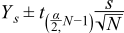
Where, Ys is the sample mean, s is the sample standard deviation, N is the sample size, /α/ is the desired significance level and t(α/2,N-1) is the upper critical value of the Students-t distribution with N-1 degrees of freedom.
![[Note]](../../../../../../../../../../doc/src/images/note.png) |
Note |
|---|---|
|
The quantity α is the maximum acceptable risk of falsely rejecting the null-hypothesis. The smaller the value of α the greater the strength of the test. The confidence level of the test is defined as 1 - α, and often expressed as a percentage. So for example a significance level of 0.05, is equivalent to a 95% confidence level. Refer to "What are confidence intervals?" in NIST/SEMATECH e-Handbook of Statistical Methods. for more information. |
|
Note |
|---|---|
The usual assumptions of independent and identically distributed (i.i.d.) variables and normal distribution of course apply here, as they do in other examples. |
From the formula, it should be clear that:
The following example code is taken from the example program students_t_single_sample.cpp.
We'll begin by defining a procedure to calculate intervals for various confidence levels; the procedure will print these out as a table:
// Needed includes:
#include <boost/math/distributions/students_t.hpp>
#include <iostream>
#include <iomanip>
// Bring everything into global namespace for ease of use:
using namespace boost::math;
using namespace std;

void confidence_limits_on_mean(
   double Sm,           // Sm = Sample Mean.
   double Sd,           // Sd = Sample Standard Deviation.
   unsigned Sn)         // Sn = Sample Size.
{
   using namespace std;
   using namespace boost::math;

   // Print out general info:
   cout <<
      "__________________________________\n"
      "2-Sided Confidence Limits For Mean\n"
      "__________________________________\n\n";
   cout << setprecision(7);
   cout << setw(40) << left << "Number of Observations" << "=  " << Sn << "\n";
   cout << setw(40) << left << "Mean" << "=  " << Sm << "\n";
   cout << setw(40) << left << "Standard Deviation" << "=  " << Sd << "\n";
We'll define a table of significance/risk levels for which we'll compute intervals:
double alpha[] = { 0.5, 0.25, 0.1, 0.05, 0.01, 0.001, 0.0001, 0.00001 };
Note that these are the complements of the confidence/probability levels: 0.5, 0.75, 0.9 .. 0.99999).
Next we'll declare the distribution object we'll need, note that the degrees of freedom parameter is the sample size less one:
students_t dist(Sn - 1);
Most of what follows in the program is pretty printing, so let's focus on the calculation of the interval. First we need the t-statistic, computed using the quantile function and our significance level. Note that since the significance levels are the complement of the probability, we have to wrap the arguments in a call to complement(...):
double T = quantile(complement(dist, alpha[i] / 2));
Note that alpha was divided by two, since we'll be calculating both the upper and lower bounds: had we been interested in a single sided interval then we would have omitted this step.
Now to complete the picture, we'll get the (one-sided) width of the interval from the t-statistic by multiplying by the standard deviation, and dividing by the square root of the sample size:
double w = T * Sd / sqrt(double(Sn));
The two-sided interval is then the sample mean plus and minus this width.
And apart from some more pretty-printing that completes the procedure.
Let's take a look at some sample output, first using the Heat flow data from the NIST site. The data set was collected by Bob Zarr of NIST in January, 1990 from a heat flow meter calibration and stability analysis. The corresponding dataplot output for this test can be found in section 3.5.2 of the NIST/SEMATECH e-Handbook of Statistical Methods..
   __________________________________
   2-Sided Confidence Limits For Mean
   __________________________________

   Number of Observations                  =  195
   Mean                                    =  9.26146
   Standard Deviation                      =  0.02278881


   ___________________________________________________________________
   Confidence       T           Interval          Lower          Upper
    Value (%)     Value          Width            Limit          Limit
   ___________________________________________________________________
       50.000     0.676       1.103e-003        9.26036        9.26256
       75.000     1.154       1.883e-003        9.25958        9.26334
       90.000     1.653       2.697e-003        9.25876        9.26416
       95.000     1.972       3.219e-003        9.25824        9.26468
       99.000     2.601       4.245e-003        9.25721        9.26571
       99.900     3.341       5.453e-003        9.25601        9.26691
       99.990     3.973       6.484e-003        9.25498        9.26794
       99.999     4.537       7.404e-003        9.25406        9.26886
As you can see the large sample size (195) and small standard deviation (0.023) have combined to give very small intervals, indeed we can be very confident that the true mean is 9.2.
For comparison the next example data output is taken from P.K.Hou, O. W. Lau & M.C. Wong, Analyst (1983) vol. 108, p 64. and from Statistics for Analytical Chemistry, 3rd ed. (1994), pp 54-55 J. C. Miller and J. N. Miller, Ellis Horwood ISBN 0 13 0309907. The values result from the determination of mercury by cold-vapour atomic absorption.
   __________________________________
   2-Sided Confidence Limits For Mean
   __________________________________

   Number of Observations                  =  3
   Mean                                    =  37.8000000
   Standard Deviation                      =  0.9643650


   ___________________________________________________________________
   Confidence       T           Interval          Lower          Upper
    Value (%)     Value          Width            Limit          Limit
   ___________________________________________________________________
       50.000     0.816            0.455       37.34539       38.25461
       75.000     1.604            0.893       36.90717       38.69283
       90.000     2.920            1.626       36.17422       39.42578
       95.000     4.303            2.396       35.40438       40.19562
       99.000     9.925            5.526       32.27408       43.32592
       99.900    31.599           17.594       20.20639       55.39361
       99.990    99.992           55.673      -17.87346       93.47346
       99.999   316.225          176.067     -138.26683      213.86683
This time the fact that there are only three measurements leads to much wider intervals, indeed such large intervals that it's hard to be very confident in the location of the mean.