 Boost
C++ Libraries
...one of the most highly
regarded and expertly designed C++ library projects in the
world.
— Herb Sutter and Andrei
Alexandrescu, C++
Coding Standards
 Boost
C++ Libraries
...one of the most highly
regarded and expertly designed C++ library projects in the
world.
— Herb Sutter and Andrei
Alexandrescu, C++
Coding Standards
Discrete distributions present us with a problem when calculating the quantile: we are starting from a continuous real-valued variable - the probability - but the result (the value of the random variable) should really be discrete.
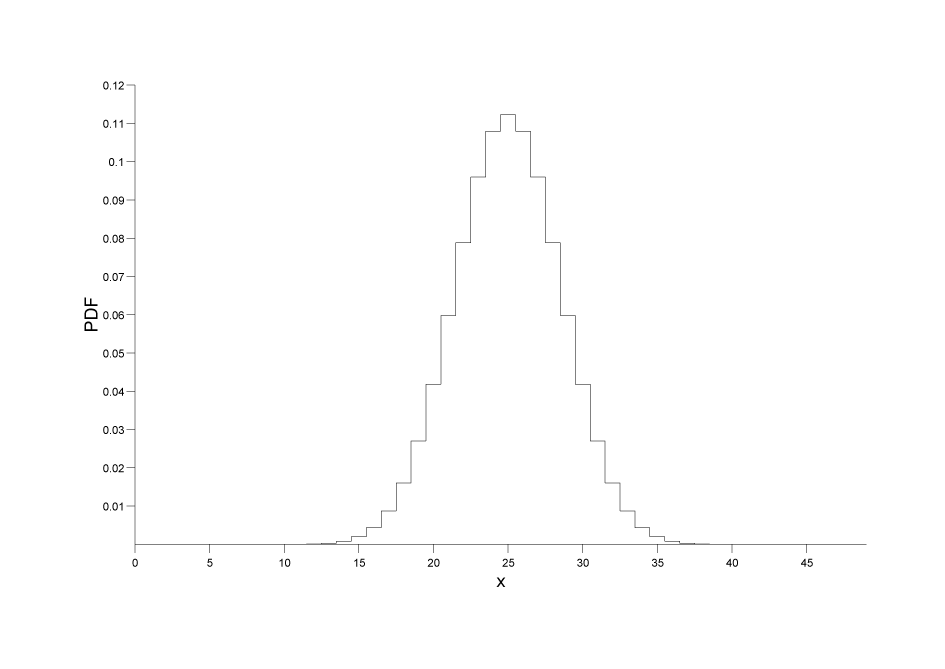
Consider for example a Binomial distribution, with a sample size of 50, and a success fraction of 0.5. There are a variety of ways we can plot a discrete distribution, but if we plot the PDF as a step-function then it looks something like this:

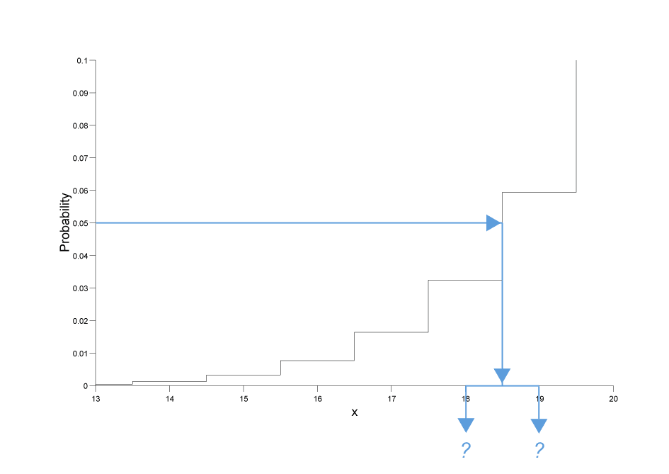
Now lets suppose that the user asks for a the quantile that corresponds to a probability of 0.05, if we zoom in on the CDF for that region here's what we see:

As can be seen there is no random variable that corresponds to a probability of exactly 0.05, so we're left with two choices as shown in the figure:
In fact there's actually a third choice as well: we could "pretend" that the distribution was continuous and return a real valued result: in this case we would calculate a result of approximately 18.701 (this accurately reflects the fact that the result is nearer to 19 than 18).
By using policies we can offer any of the above as options, but that still leaves the question: What is actually the right thing to do?
And in particular: What policy should we use by default?
In coming to an answer we should realise that:
So there is a genuine benefit to calculating an integer result as well as it being "the right thing to do" from a philosophical point of view. What's more if someone asks for a quantile at 0.05, then we can normally assume that they are asking for at least 95% of the probability to the right of the value chosen, and no more than 5% of the probability to the left of the value chosen.
In the above binomial example we would therefore round the result down to 18.
The converse applies to upper-quantiles: If the probability is greater than 0.5 we would want to round the quantile up, so that at least the requested probability is to the left of the value returned, and no more than 1 - the requested probability is to the right of the value returned.
Likewise for two-sided intervals, we would round lower quantiles down, and upper quantiles up. This ensures that we have at least the requested probability in the central region and no more than 1 minus the requested probability in the tail areas.
For example, taking our 50 sample binomial distribution with a success fraction of 0.5, if we wanted a two sided 90% confidence interval, then we would ask for the 0.05 and 0.95 quantiles with the results rounded outwards so that at least 90% of the probability is in the central area:

So far so good, but there is in fact a trap waiting for the unwary here:
quantile(binomial(50, 0.5), 0.05);
returns 18 as the result, which is what we would expect from the graph above, and indeed there is no x greater than 18 for which:
cdf(binomial(50, 0.5), x) <= 0.05;
However:
quantile(binomial(50, 0.5), 0.95);
returns 31, and indeed while there is no x less than 31 for which:
cdf(binomial(50, 0.5), x) >= 0.95;
We might naively expect that for this symmetrical distribution the result would be 32 (since 32 = 50 - 18), but we need to remember that the cdf of the binomial is inclusive of the random variable. So while the left tail area includes the quantile returned, the right tail area always excludes an upper quantile value: since that "belongs" to the central area.
Look at the graph above to see what's going on here: the lower quantile of 18 belongs to the left tail, so any value <= 18 is in the left tail. The upper quantile of 31 on the other hand belongs to the central area, so the tail area actually starts at 32, so any value > 31 is in the right tail.
Therefore if U and L are the upper and lower quantiles respectively, then a random variable X is in the tail area - where we would reject the null hypothesis if:
X <= L || X > U
And the a variable X is inside the central region if:
L < X <= U
The moral here is to always be very careful with your comparisons when dealing with a discrete distribution, and if in doubt, base your comparisons on CDF's instead.
As you would expect from a section on policies, you won't be surprised to know that other rounding options are available:
This is the default policy as described above: lower quantiles are rounded down (probability < 0.5), and upper quantiles (probability > 0.5) are rounded up.
This gives no more than the requested probability in the tails, and at least the requested probability in the central area.
This is the exact opposite of the default policy: lower quantiles are rounded up (probability < 0.5), and upper quantiles (probability > 0.5) are rounded down.
This gives at least the requested probability in the tails, and no more than the requested probability in the central area.
This policy will always round the result down no matter whether it is an upper or lower quantile
This policy will always round the result up no matter whether it is an upper or lower quantile
This policy will always round the result to the nearest integer no matter whether it is an upper or lower quantile
This policy will return a real valued result for the quantile of a discrete distribution: this is generally much slower than finding an integer result but does allow for more sophisticated rounding policies.
To understand how the rounding policies for the discrete distributions can be used, we'll use the 50-sample binomial distribution with a success fraction of 0.5 once again, and calculate all the possible quantiles at 0.05 and 0.95.
Begin by including the needed headers (and some using statements for conciseness):
#include <iostream>
using std::cout; using std::endl;
using std::left; using std::fixed; using std::right; using std::scientific;
#include <iomanip>
using std::setw;
using std::setprecision;

#include <boost/math/distributions/binomial.hpp>
Next we'll bring the needed declarations into scope, and define distribution types for all the available rounding policies:
// Avoid
// using namespace std; // and
// using namespace boost::math;
// to avoid potential ambiguity of names, like binomial.
// using namespace boost::math::policies; is small risk, but
// the necessary items are brought into scope thus:

using boost::math::binomial_distribution;
using boost::math::policies::policy;
using boost::math::policies::discrete_quantile;

using boost::math::policies::integer_round_outwards;
using boost::math::policies::integer_round_down;
using boost::math::policies::integer_round_up;
using boost::math::policies::integer_round_nearest;
using boost::math::policies::integer_round_inwards;
using boost::math::policies::real;

using boost::math::binomial_distribution; // Not std::binomial_distribution.

typedef binomial_distribution<
            double,
            policy<discrete_quantile<integer_round_outwards> > >
        binom_round_outwards;

typedef binomial_distribution<
            double,
            policy<discrete_quantile<integer_round_inwards> > >
        binom_round_inwards;

typedef binomial_distribution<
            double,
            policy<discrete_quantile<integer_round_down> > >
        binom_round_down;

typedef binomial_distribution<
            double,
            policy<discrete_quantile<integer_round_up> > >
        binom_round_up;

typedef binomial_distribution<
            double,
            policy<discrete_quantile<integer_round_nearest> > >
        binom_round_nearest;

typedef binomial_distribution<
            double,
            policy<discrete_quantile<real> > >
        binom_real_quantile;
Now let's set to work calling those quantiles:
int main()
{
   cout <<
      "Testing rounding policies for a 50 sample binomial distribution,\n"
      "with a success fraction of 0.5.\n\n"
      "Lower quantiles are calculated at p = 0.05\n\n"
      "Upper quantiles at p = 0.95.\n\n";

   cout << setw(25) << right
      << "Policy"<< setw(18) << right
      << "Lower Quantile" << setw(18) << right
      << "Upper Quantile" << endl;

   // Test integer_round_outwards:
   cout << setw(25) << right
      << "integer_round_outwards"
      << setw(18) << right
      << quantile(binom_round_outwards(50, 0.5), 0.05)
      << setw(18) << right
      << quantile(binom_round_outwards(50, 0.5), 0.95)
      << endl;

   // Test integer_round_inwards:
   cout << setw(25) << right
      << "integer_round_inwards"
      << setw(18) << right
      << quantile(binom_round_inwards(50, 0.5), 0.05)
      << setw(18) << right
      << quantile(binom_round_inwards(50, 0.5), 0.95)
      << endl;

   // Test integer_round_down:
   cout << setw(25) << right
      << "integer_round_down"
      << setw(18) << right
      << quantile(binom_round_down(50, 0.5), 0.05)
      << setw(18) << right
      << quantile(binom_round_down(50, 0.5), 0.95)
      << endl;

   // Test integer_round_up:
   cout << setw(25) << right
      << "integer_round_up"
      << setw(18) << right
      << quantile(binom_round_up(50, 0.5), 0.05)
      << setw(18) << right
      << quantile(binom_round_up(50, 0.5), 0.95)
      << endl;

   // Test integer_round_nearest:
   cout << setw(25) << right
      << "integer_round_nearest"
      << setw(18) << right
      << quantile(binom_round_nearest(50, 0.5), 0.05)
      << setw(18) << right
      << quantile(binom_round_nearest(50, 0.5), 0.95)
      << endl;

   // Test real:
   cout << setw(25) << right
      << "real"
      << setw(18) << right
      << quantile(binom_real_quantile(50, 0.5), 0.05)
      << setw(18) << right
      << quantile(binom_real_quantile(50, 0.5), 0.95)
      << endl;
} // int main()
Which produces the program output:
  policy_eg_10.vcxproj -> J:\Cpp\MathToolkit\test\Math_test\Release\policy_eg_10.exe
  Testing rounding policies for a 50 sample binomial distribution,
  with a success fraction of 0.5.

  Lower quantiles are calculated at p = 0.05

  Upper quantiles at p = 0.95.

                     Policy    Lower Quantile    Upper Quantile
     integer_round_outwards                18                31
      integer_round_inwards                19                30
         integer_round_down                18                30
           integer_round_up                19                31
      integer_round_nearest                19                30
                       real            18.701            30.299