#include <boost/math/distributions/poisson.hpp>
namespace boost { namespace math {
template <class RealType = double,
class Policy = policies::policy<> >
class poisson_distribution;
typedef poisson_distribution<> poisson;
template <class RealType, class Policy>
class poisson_distribution
{
public:
typedef RealType value_type;
typedef Policy policy_type;
poisson_distribution(RealType mean = 1); RealType mean()const; }
}}
The Poisson
distribution is a well-known statistical discrete distribution.
It expresses the probability of a number of events (or failures, arrivals,
occurrences ...) occurring in a fixed period of time, provided these
events occur with a known mean rate λ
(events/time), and are independent
of the time since the last event.
The distribution was discovered by Simé on-Denis Poisson (1781 to 1840).
It has the Probability Mass Function:

for k events, with an expected number of events λ.
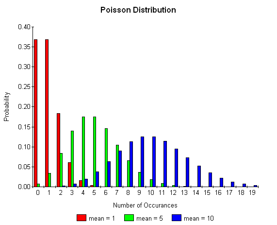
The following graph illustrates how the PDF varies with the parameter
λ:
![[Caution]](../../../../../../../../../doc/html/images/caution.png) |
Caution |
|
The Poisson distribution is a discrete distribution: internally functions
like the cdf and
pdf are treated "as
if" they are continuous functions, but in reality the results
returned from these functions only have meaning if an integer value
is provided for the random variate argument.
The quantile function will by default return an integer result that
has been rounded outwards. That is to say lower
quantiles (where the probability is less than 0.5) are rounded downward,
and upper quantiles (where the probability is greater than 0.5) are
rounded upwards. This behaviour ensures that if an X% quantile is
requested, then at least the requested coverage
will be present in the central region, and no more than
the requested coverage will be present in the tails.
This behaviour can be changed so that the quantile functions are
rounded differently, or even return a real-valued result using Policies. It is
strongly recommended that you read the tutorial Understanding
Quantiles of Discrete Distributions before using the quantile
function on the Poisson distribution. The reference
docs describe how to change the rounding policy for these
distributions.
|
poisson_distribution(RealType mean = 1);
Constructs a poisson distribution with mean mean.
RealType mean()const;
Returns the mean of this distribution.
All the usual non-member
accessor functions that are generic to all distributions are supported:
Cumulative Distribution Function,
Probability Density Function, Quantile, Hazard
Function, Cumulative Hazard Function,
mean, median,
mode, variance,
standard deviation, skewness,
kurtosis, kurtosis_excess,
range and support.
The domain of the random variable is [0, ∞].
The Poisson distribution is implemented in terms of the incomplete gamma
functions gamma_p
and gamma_q
and as such should have low error rates: but refer to the documentation
of those functions for more information. The quantile and its complement
use the inverse gamma functions and are therefore probably slightly less
accurate: this is because the inverse gamma functions are implemented
using an iterative method with a lower tolerance to avoid excessive computation.
In the following table λ is the mean of the distribution, k
is the random variable, p is the probability and
q = 1-p.
 Boost
C++ Libraries
Boost
C++ Libraries


